#Please install all packages not already installed using
#a command similar to one below
#install.packages("dslabs")

library(dslabs) #How we will access the dataset
library(tidyr) #For cleaning and analyzing the data
library(dplyr) #For creating pipes to sort, filter data
library(ggplot2) # For creating nice visuals
library(scales) # For scaling data R Coding Exercise
Analyzing Life Expectancy in Africa
We will be using data from the Gapminder package in R
Taking a look at the structure of the data
# This will give us dimensions and column details
str(gapminder)
'data.frame': 10545 obs. of 9 variables:
$ country : Factor w/ 185 levels "Albania","Algeria",..: 1 2 3 4 5 6 7 8 9 10 ...
$ year : int 1960 1960 1960 1960 1960 1960 1960 1960 1960 1960 ...
$ infant_mortality: num 115.4 148.2 208 NA 59.9 ...
$ life_expectancy : num 62.9 47.5 36 63 65.4 ...
$ fertility : num 6.19 7.65 7.32 4.43 3.11 4.55 4.82 3.45 2.7 5.57 ...
$ population : num 1636054 11124892 5270844 54681 20619075 ...
$ gdp : num NA 1.38e+10 NA NA 1.08e+11 ...
$ continent : Factor w/ 5 levels "Africa","Americas",..: 4 1 1 2 2 3 2 5 4 3 ...
$ region : Factor w/ 22 levels "Australia and New Zealand",..: 19 11 10 2 15 21 2 1 22 21 ...Assessing the quartiles for each column
#This will give us an idea of how each column's data is spread out, and give us some insight about outliers
summary(gapminder)
country year infant_mortality life_expectancy
Albania : 57 Min. :1960 Min. : 1.50 Min. :13.20
Algeria : 57 1st Qu.:1974 1st Qu.: 16.00 1st Qu.:57.50
Angola : 57 Median :1988 Median : 41.50 Median :67.54
Antigua and Barbuda: 57 Mean :1988 Mean : 55.31 Mean :64.81
Argentina : 57 3rd Qu.:2002 3rd Qu.: 85.10 3rd Qu.:73.00
Armenia : 57 Max. :2016 Max. :276.90 Max. :83.90
(Other) :10203 NA's :1453
fertility population gdp continent
Min. :0.840 Min. :3.124e+04 Min. :4.040e+07 Africa :2907
1st Qu.:2.200 1st Qu.:1.333e+06 1st Qu.:1.846e+09 Americas:2052
Median :3.750 Median :5.009e+06 Median :7.794e+09 Asia :2679
Mean :4.084 Mean :2.701e+07 Mean :1.480e+11 Europe :2223
3rd Qu.:6.000 3rd Qu.:1.523e+07 3rd Qu.:5.540e+10 Oceania : 684
Max. :9.220 Max. :1.376e+09 Max. :1.174e+13
NA's :187 NA's :185 NA's :2972
region
Western Asia :1026
Eastern Africa : 912
Western Africa : 912
Caribbean : 741
South America : 684
Southern Europe: 684
(Other) :5586 Verifying the type of object that we will be accesssing
class(gapminder)[1] "data.frame"# Tells us that R is viewing this as a data frame which will help us with maintaining column types and cleaning the datasetProcessing data
First we will segment only data from African countries into a new data frame.
# Using pipes from dplyr
africadata = gapminder |>
  filter(continent == 'Africa') # Using two == signifies comparison operator vs assignment operator
Next we will create two new objects from this Africa data set, one with both Life Expectancy and Infant Mortality, and one with both Life Expectancy and Population.
africa_IM_LE = africadata[3:4] #Slicing only two columns of interest
africa_POP_LE = africadata[4:6] #Slicing three columns since we want both 4 and 6
africa_POP_LE = africa_POP_LE[-2] #Removing middle unneeded columns
Lets take a look at the structure and summary of the two new data objects.
str(africa_POP_LE)'data.frame': 2907 obs. of 2 variables:
$ life_expectancy: num 47.5 36 38.3 50.3 35.2 ...
$ population : num 11124892 5270844 2431620 524029 4829291 ...str(africa_IM_LE)'data.frame': 2907 obs. of 2 variables:
$ infant_mortality: num 148 208 187 116 161 ...
$ life_expectancy : num 47.5 36 38.3 50.3 35.2 ...summary(africa_POP_LE) life_expectancy population
Min. :13.20 Min. : 41538
1st Qu.:48.23 1st Qu.: 1605232
Median :53.98 Median : 5570982
Mean :54.38 Mean : 12235961
3rd Qu.:60.10 3rd Qu.: 13888152
Max. :77.60 Max. :182201962
NA's :51 summary(africa_IM_LE) infant_mortality life_expectancy
Min. : 11.40 Min. :13.20
1st Qu.: 62.20 1st Qu.:48.23
Median : 93.40 Median :53.98
Mean : 95.12 Mean :54.38
3rd Qu.:124.70 3rd Qu.:60.10
Max. :237.40 Max. :77.60
NA's :226 Plotting
Plotting Life Expectancy as function of Infant Mortality.
africa_IM_LE |> # Using pipes again
  ggplot(aes(x=infant_mortality, y=life_expectancy))+ #Using GGplot for better visualizations
  geom_point() #geom_point is ggplots method for scatterplots
Warning: Removed 226 rows containing missing values or values outside the scale range
(`geom_point()`).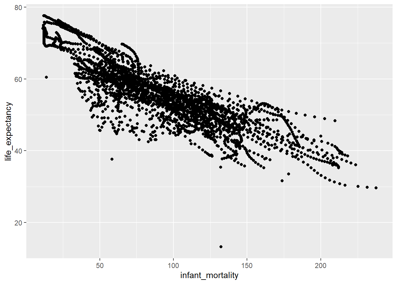
We can clearly see a negative correlation between our variables of interest, implying as infant mortality increases, life expectancy decreases.
Next plotting Life Expectancy as a function of Population
africa_POP_LE |>
  ggplot(aes(x = population, y =life_expectancy))+
  geom_point()+
  scale_x_log10(labels = label_comma()) #Using the scales library to scale the x axis with log10
Warning: Removed 51 rows containing missing values or values outside the scale range
(`geom_point()`).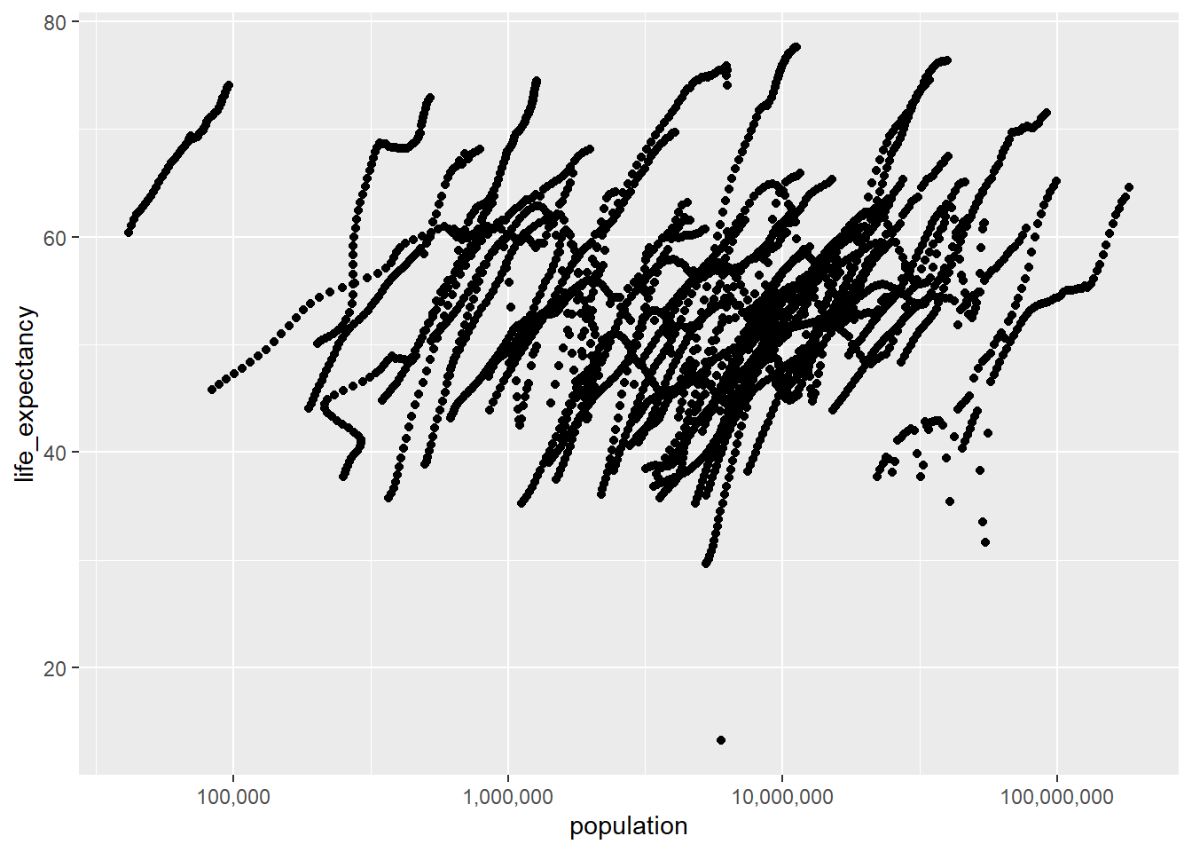
We generally see a positive correlation between these two variables. As in the previous plot we can note several ‘lines’ of data made up of datapoints very close to each other. These represent the data of distinct countries, year after year, increasing or decreasing.
Additional Data Processing
We need find a a singular year to explore.
In order to do that, we need to identify which years are not missing data for the Infant Mortality variable.
#We start by counting the number of NAs per country, per year
CountNAs = africadata |>
  group_by(year) |> # When we group, we need to summarize
  summarise(sum(is.na(infant_mortality)))#so we use the total number of NA values in this column to group on

CountNAs #Generating table
# A tibble: 57 × 2
year `sum(is.na(infant_mortality))`
<int> <int>
1 1960 10
2 1961 17
3 1962 16
4 1963 16
5 1964 15
6 1965 14
7 1966 13
8 1967 11
9 1968 11
10 1969 7
# ℹ 47 more rows#Clicking through the table will show when the number of NAs drop to 0 for many years
plot(CountNAs) # Plotting our findings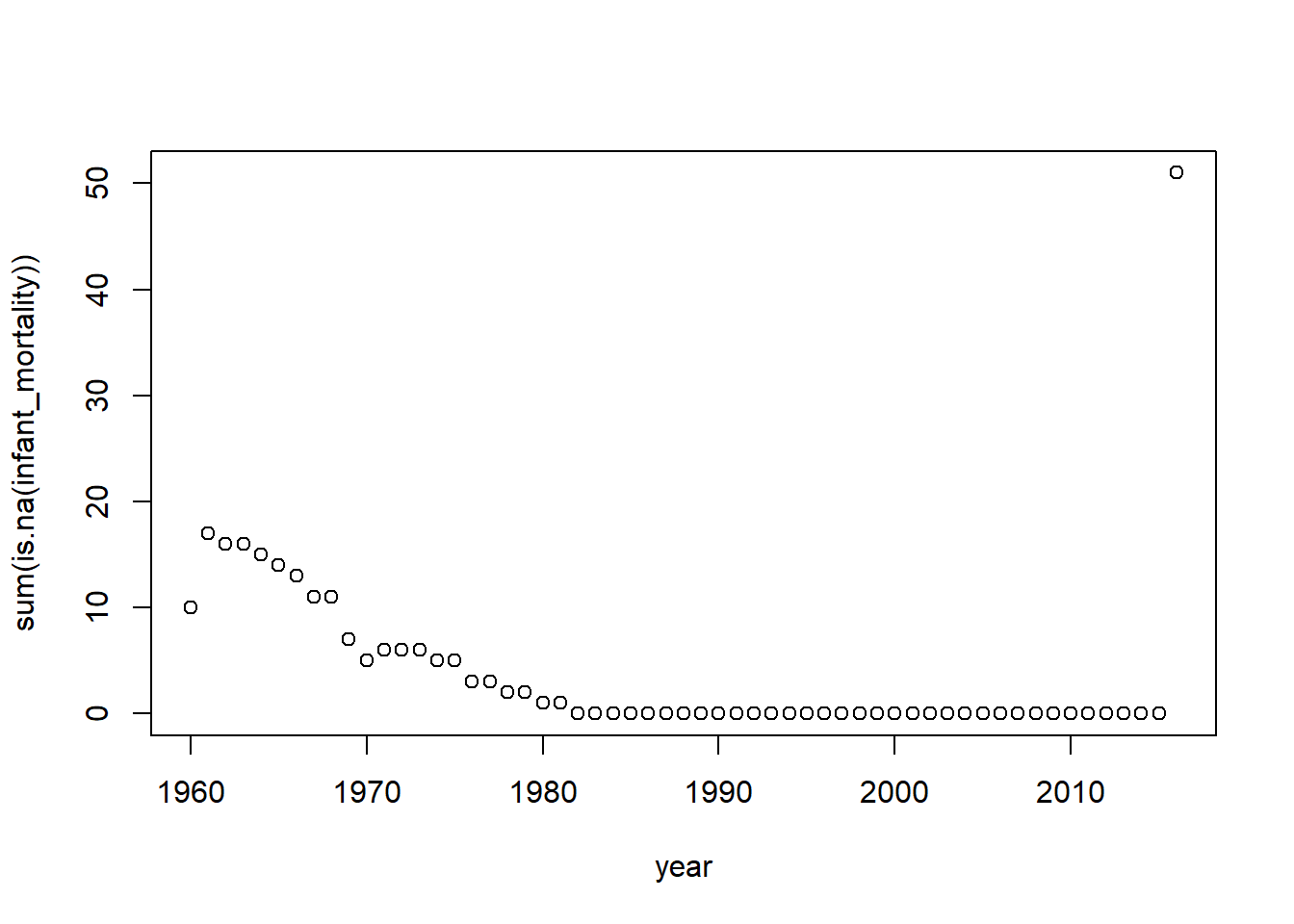
As both the table and plot show, around 1981, the number of NAs for the Infant Mortality variable dropped to 0 until 2016, when the number of NAs jumped. So we need to choose a year between that year range.We will choose 2000 for this exercise.
# Creating a new data object
africa2000 = africadata |>
  filter(year == 2000)# We only want rows where the year column is 2000


# Checking both the structure and summary of our new data object

str(africa2000)
'data.frame': 51 obs. of 9 variables:
$ country : Factor w/ 185 levels "Albania","Algeria",..: 2 3 18 22 26 27 29 31 32 33 ...
$ year : int 2000 2000 2000 2000 2000 2000 2000 2000 2000 2000 ...
$ infant_mortality: num 33.9 128.3 89.3 52.4 96.2 ...
$ life_expectancy : num 73.3 52.3 57.2 47.6 52.6 46.7 54.3 68.4 45.3 51.5 ...
$ fertility : num 2.51 6.84 5.98 3.41 6.59 7.06 5.62 3.7 5.45 7.35 ...
$ population : num 31183658 15058638 6949366 1736579 11607944 ...
$ gdp : num 5.48e+10 9.13e+09 2.25e+09 5.63e+09 2.61e+09 ...
$ continent : Factor w/ 5 levels "Africa","Americas",..: 1 1 1 1 1 1 1 1 1 1 ...
$ region : Factor w/ 22 levels "Australia and New Zealand",..: 11 10 20 17 20 5 10 20 10 10 ...summary(africa2000) country year infant_mortality life_expectancy
Algeria : 1 Min. :2000 Min. : 12.30 Min. :37.60
Angola : 1 1st Qu.:2000 1st Qu.: 60.80 1st Qu.:51.75
Benin : 1 Median :2000 Median : 80.30 Median :54.30
Botswana : 1 Mean :2000 Mean : 78.93 Mean :56.36
Burkina Faso: 1 3rd Qu.:2000 3rd Qu.:103.30 3rd Qu.:60.00
Burundi : 1 Max. :2000 Max. :143.30 Max. :75.00
(Other) :45
fertility population gdp continent
Min. :1.990 Min. : 81154 Min. :2.019e+08 Africa :51
1st Qu.:4.150 1st Qu.: 2304687 1st Qu.:1.274e+09 Americas: 0
Median :5.550 Median : 8799165 Median :3.238e+09 Asia : 0
Mean :5.156 Mean : 15659800 Mean :1.155e+10 Europe : 0
3rd Qu.:5.960 3rd Qu.: 17391242 3rd Qu.:8.654e+09 Oceania : 0
Max. :7.730 Max. :122876723 Max. :1.329e+11
region
Eastern Africa :16
Western Africa :16
Middle Africa : 8
Northern Africa : 6
Southern Africa : 5
Australia and New Zealand: 0
(Other) : 0 Additional Plotting
Now, lets generate the same plots from before, with just data from Africa in the year 2000.
Plotting Life Expectancy as function of Infant Mortality
africa2000 |> # Our new data object
  ggplot(aes(x=infant_mortality, y=life_expectancy))+
  geom_point()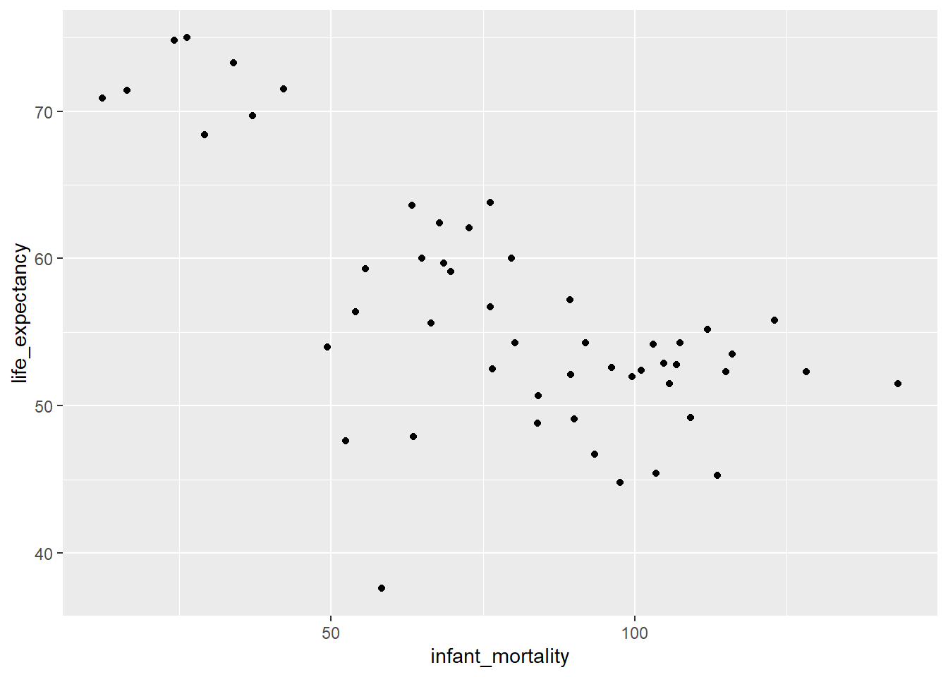
We still see the same negative correlation as before, albeit less strong.
Next plotting Life Expectancy as a function of Population
africa2000 |>
  ggplot(aes(x = population, y =life_expectancy))+
  geom_point()+
  scale_x_log10(labels = label_comma()) #Using Scales again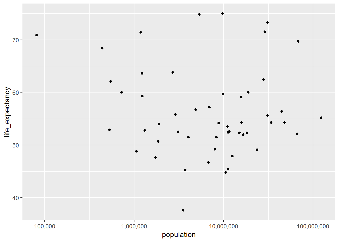
We do not see a real trend in this plot, which differs from the initial plot with all the data from African.
Modeling
We will fit two models using two different predictors (infant mortality and population) to predict life expectancy.
fit1 = lm(life_expectancy ~ infant_mortality, data=africa2000) # Initializing model using infant_mortality as predictor

fit2 =lm(life_expectancy ~ population, data=africa2000)
#Model using Population as predictor
Now we run summary() to display the results of our two model runs.
summary(fit1) #Summary will show us all the important info of our two models
Call:
lm(formula = life_expectancy ~ infant_mortality, data = africa2000)

Residuals:
     Min       1Q   Median       3Q      Max
-22.6651  -3.7087   0.9914   4.0408   8.6817

Coefficients:
                 Estimate Std. Error t value Pr(>|t|)
(Intercept)      71.29331    2.42611  29.386  < 2e-16 ***
infant_mortality -0.18916    0.02869  -6.594 2.83e-08 ***
---
Signif. codes:  0 '***' 0.001 '**' 0.01 '*' 0.05 '.' 0.1 ' ' 1

Residual standard error: 6.221 on 49 degrees of freedom
Multiple R-squared:  0.4701,    Adjusted R-squared:  0.4593
F-statistic: 43.48 on 1 and 49 DF, p-value: 2.826e-08summary(fit2)
Call:
lm(formula = life_expectancy ~ population, data = africa2000)

Residuals:
    Min      1Q  Median      3Q     Max
-18.429  -4.602  -2.568   3.800  18.802

Coefficients:
             Estimate Std. Error t value Pr(>|t|)
(Intercept) 5.593e+01  1.468e+00  38.097   <2e-16 ***
population  2.756e-08  5.459e-08   0.505    0.616
---
Signif. codes:  0 '***' 0.001 '**' 0.01 '*' 0.05 '.' 0.1 ' ' 1

Residual standard error: 8.524 on 49 degrees of freedom
Multiple R-squared:  0.005176,  Adjusted R-squared:  -0.01513
F-statistic: 0.2549 on 1 and 49 DF,  p-value: 0.6159
Model Conclusions
As expected model 1 (Predictor: Infant Mortality) has a significant effect (p-value is far below .05), and that effect is negative (intercept is -.1891).
Also as expected, model 2 (Predictor: Population) did not have a substantial effect (p-value .6 > .05).