library(tidyr)
library(here)
library(synthpop) # Primary library needed for creating Synthetic Data
library(performance) # Using this to test models and compare models
library(see) #Needed to supplement the above library
library(corrplot) # Used for Correlation PlotSynthetic Data Project
Reading in the Data
I chose a health data set with different bio variables like BMI and Blood Pressure.
data_location <- here("synthetic-data-exercise","Healthcare-Diabetes.csv")

rawdata <- read.csv(data_location, sep = ",")
Before generating new data set
We want to create some models to test with both data sets. Even thought the synthetic data will have different data than our original dataset, the results from the models should remain close to the same.
#Using BMI as outcome with Glucose, BP, and Age as predictors
fit1 = lm(BMI ~  Glucose + BloodPressure + Age,
          data=rawdata)

(results = summary(fit1))
Call:
lm(formula = BMI ~ Glucose + BloodPressure + Age, data = rawdata)

Residuals:
    Min      1Q  Median      3Q     Max
-34.258  -4.830  -0.362   4.587  45.961

Coefficients:
               Estimate Std. Error t value Pr(>|t|)
(Intercept)   19.750111   0.741469  26.636  < 2e-16 ***
Glucose        0.052255   0.004672  11.185  < 2e-16 ***
BloodPressure  0.113870   0.007745  14.703  < 2e-16 ***
Age           -0.054728   0.012953  -4.225 2.47e-05 ***
---
Signif. codes:  0 '***' 0.001 '**' 0.01 '*' 0.05 '.' 0.1 ' ' 1

Residual standard error: 7.58 on 2764 degrees of freedom
Multiple R-squared:   0.12, Adjusted R-squared:  0.119
F-statistic: 125.6 on 3 and 2764 DF,  p-value: < 2.2e-16
fit2 = lm(BMI ~ Glucose + BloodPressure + Age,
data=rawdata)
(summary(fit2))
Call:
lm(formula = BMI ~ Glucose + BloodPressure + Age, data = rawdata)

Residuals:
    Min      1Q  Median      3Q     Max
-34.258  -4.830  -0.362   4.587  45.961

Coefficients:
               Estimate Std. Error t value Pr(>|t|)
(Intercept)   19.750111   0.741469  26.636  < 2e-16 ***
Glucose        0.052255   0.004672  11.185  < 2e-16 ***
BloodPressure  0.113870   0.007745  14.703  < 2e-16 ***
Age           -0.054728   0.012953  -4.225 2.47e-05 ***
---
Signif. codes:  0 '***' 0.001 '**' 0.01 '*' 0.05 '.' 0.1 ' ' 1

Residual standard error: 7.58 on 2764 degrees of freedom
Multiple R-squared:   0.12, Adjusted R-squared:  0.119
F-statistic: 125.6 on 3 and 2764 DF,  p-value: < 2.2e-16
Discovered this incredibly useful took for visually assessing your model.
check_model(fit1)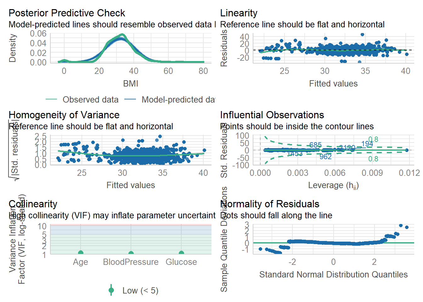
check_model(fit2)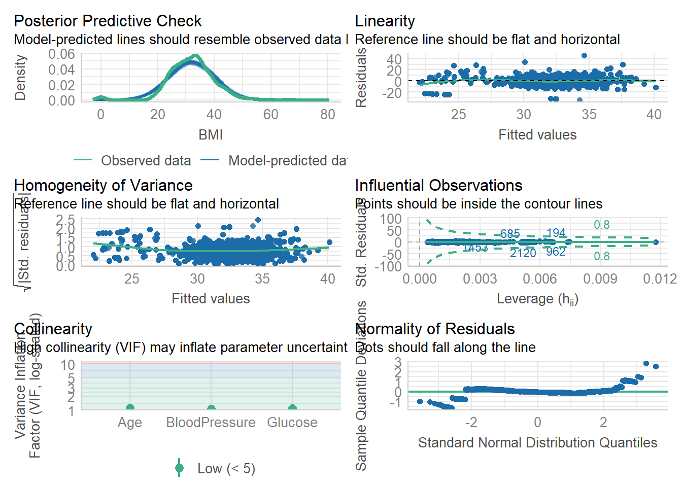
Both of our models look visually solid. Our prediction lines follows the observed data lines, and our residuals roughly fall long the normality line.
Modifying data slightly
rawdata$Outcome = as.factor(rawdata$Outcome)
codebook.syn(rawdata)
$tab
variable class nmiss perctmiss ndistinct
1 Id integer 0 0 2768
2 Pregnancies integer 0 0 17
3 Glucose integer 0 0 136
4 BloodPressure integer 0 0 47
5 SkinThickness integer 0 0 53
6 Insulin integer 0 0 187
7 BMI numeric 0 0 253
8 DiabetesPedigreeFunction numeric 0 0 523
9 Age integer 0 0 52
10 Outcome factor 0 0 2
details
1
2
3
4
5
6
7 Range: 0 - 80.6
8 Range: 0.078 - 2.42
9
10 '0' '1'
$labs
NULLCreating Synthetic Data
new_seed = 21 # Setting our seed at a random value
synthetic_data = syn(rawdata,
                     seed = new_seed) #This will give us our synthetic dataset
Synthesis
-----------
 Id Pregnancies Glucose BloodPressure SkinThickness Insulin BMI DiabetesPedigreeFunction Age Outcome
#cleaning the synthetic dataset
synth_data_clean = sdc(synthetic_data, rawdata,
label = "FAKE DATA",
rm.replicated.uniques = TRUE) #This is important! Sometimes, when we create "fake" synthetic data, we happen to recreate an actual observation in the original data set. So, in the name of privacy, we remove those observations.no. of replicated uniques: 4write.syn(synth_data_clean,
filename = "synthetic_diabetes_data",
filetype = "csv") #Outputting our synthetic dataSynthetic data exported as csv file(s).
Information on synthetic data written to
C:/Users/Client/Documents/antonioflores-P2-portfolio/synthetic-data-exercise/synthesis_info_synthetic_diabetes_data.txt Comparing the Data Sets
compare(synthetic_data, rawdata, stat = "counts")
Comparing counts observed with synthetic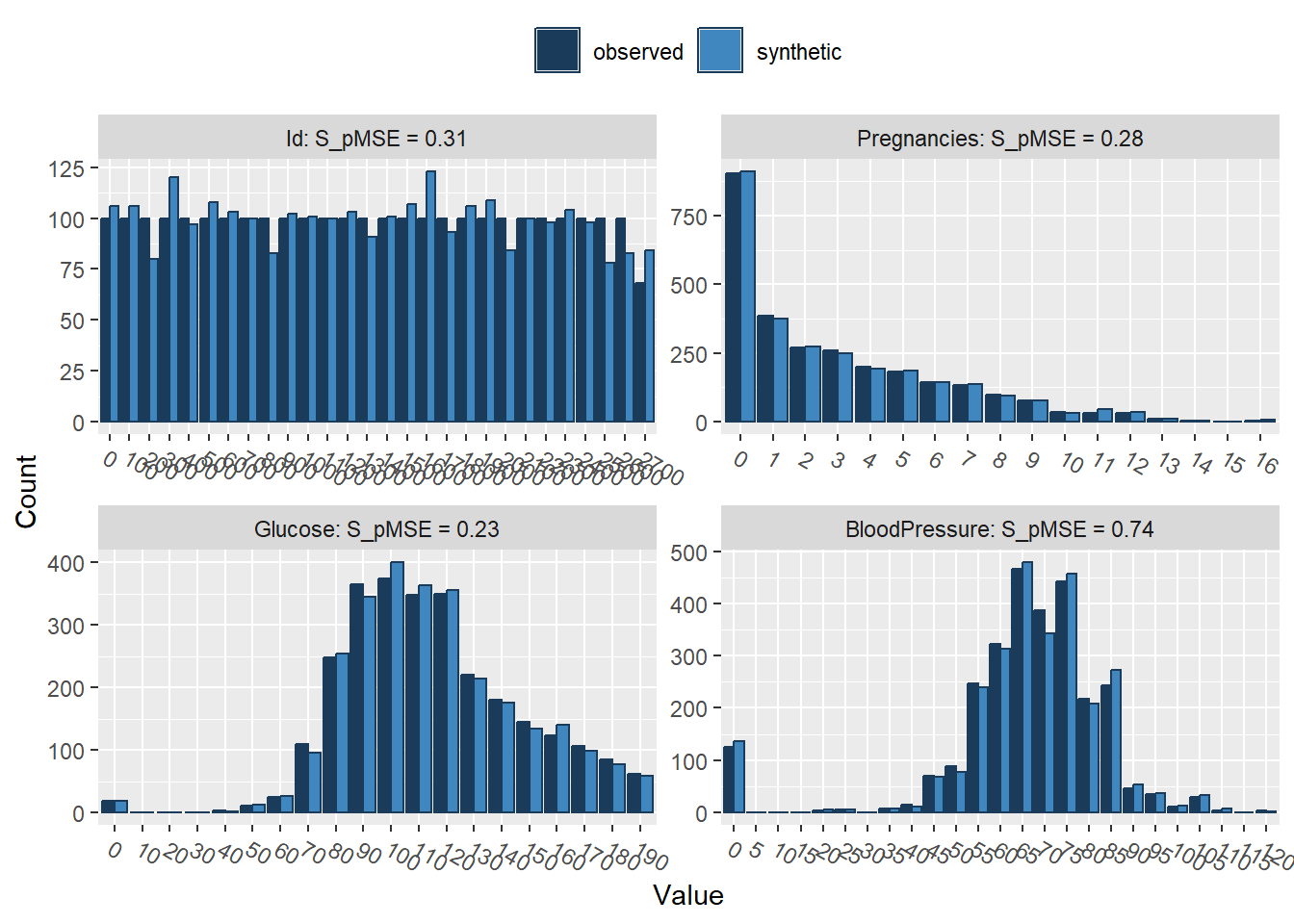
Press return for next variable(s): 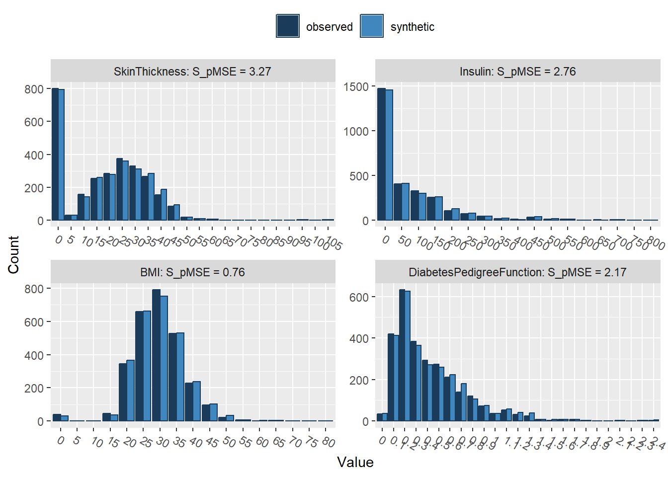
Press return for next variable(s): 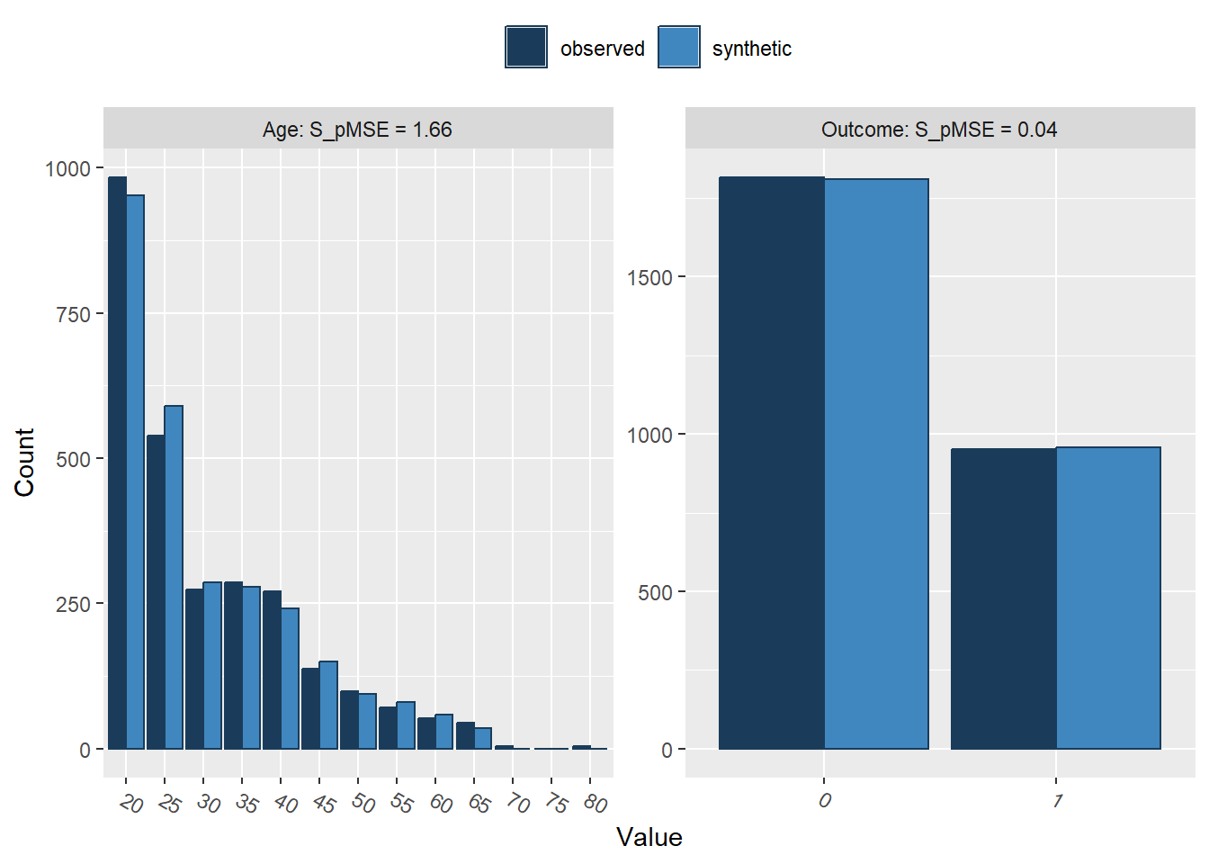
Selected utility measures:
                             pMSE   S_pMSE df
Id                       0.000028 0.309741  4
Pregnancies              0.000026 0.283048  4
Glucose                  0.000021 0.229948  4
BloodPressure            0.000067 0.738437  4
SkinThickness            0.000222 3.271697  3
Insulin                  0.000125 2.757808  2
BMI                      0.000069 0.761283  4
DiabetesPedigreeFunction 0.000196 2.174107  4
Age                      0.000150 1.657246  4
Outcome                  0.000001 0.039977  1
We can easily see that the synthetic dataset (light blue) closely resembles our original data set (dark blue)
Testing associations
synth_fit = lm.synds(BMI ~  Glucose + BloodPressure + Age,
          data=synthetic_data)

compare(synth_fit, rawdata)
Call used to fit models to the data:
lm.synds(formula = BMI ~ Glucose + BloodPressure + Age, data = synthetic_data)

Differences between results based on synthetic and observed data:
                Synthetic    Observed         Diff Std. coef diff CI overlap
(Intercept)   19.75878326 19.75011087  0.008672388     0.01169623  0.9970162
Glucose        0.05770880  0.05225509  0.005453708     1.16738806  0.7021914
BloodPressure  0.08994052  0.11386986 -0.023929344    -3.08970102  0.2117965
Age           -0.01893494 -0.05472831  0.035793376     2.76322362  0.2950831

Measures for one synthesis and 4 coefficients
Mean confidence interval overlap:  0.5515218
Mean absolute std. coef diff:  1.758002

Mahalanobis distance ratio for lack-of-fit (target 1.0): 4.61
Lack-of-fit test: 18.42926; p-value 0.001 for test that synthesis model is
compatible with a chi-squared test with 4 degrees of freedom.

Confidence interval plot: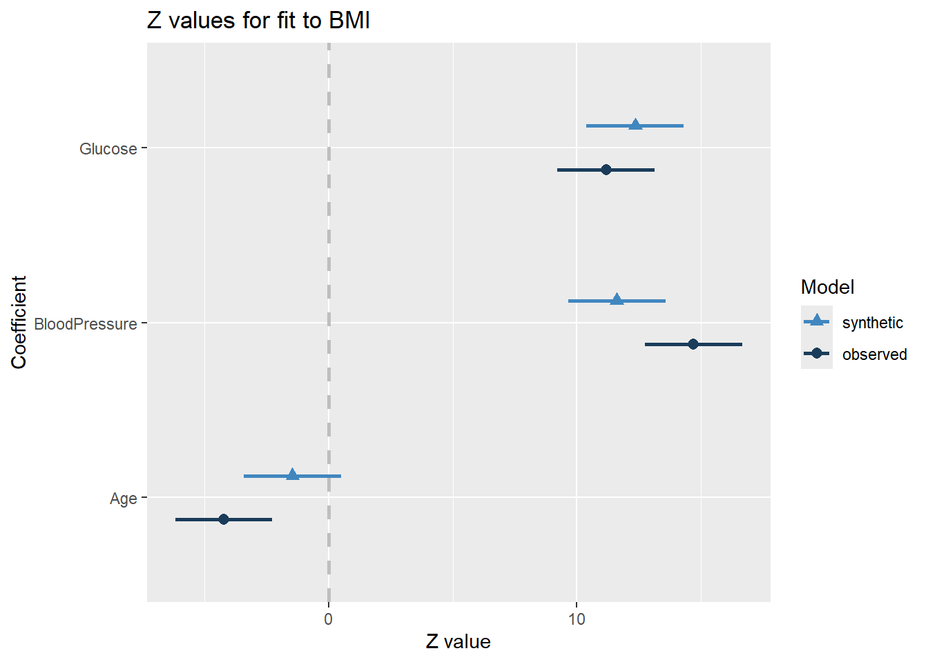
There are some differences between both data sets, but they are not significant. The P-value of this test is above .05 which in this case tells us there is not a substantial difference between the two model’s results. Assessing the visual chart we also see a fairly close similarity.
synth_fit2 = lm.synds(DiabetesPedigreeFunction ~  SkinThickness + Insulin + Pregnancies,
          data=synthetic_data)

compare(synth_fit2, rawdata)
Call used to fit models to the data:
lm.synds(formula = DiabetesPedigreeFunction ~ SkinThickness +
    Insulin + Pregnancies, data = synthetic_data)

Differences between results based on synthetic and observed data:
                  Synthetic      Observed          Diff Std. coef diff
(Intercept)    0.4199111517  0.3928253745  2.708578e-02      2.1836294
SkinThickness  0.0022171649  0.0023947366 -1.775717e-04     -0.4220489
Insulin        0.0004052427  0.0003978994  7.343269e-06      0.1219856
Pregnancies   -0.0038284710 -0.0009043188 -2.924152e-03     -1.6019283
              CI overlap
(Intercept)    0.4429415
SkinThickness  0.8923325
Insulin        0.9688807
Pregnancies    0.5913373

Measures for one synthesis and 4 coefficients
Mean confidence interval overlap:  0.723873
Mean absolute std. coef diff:  1.082398

Mahalanobis distance ratio for lack-of-fit (target 1.0): 1.84
Lack-of-fit test: 7.346747; p-value 0.1187 for test that synthesis model is
compatible with a chi-squared test with 4 degrees of freedom.

Confidence interval plot: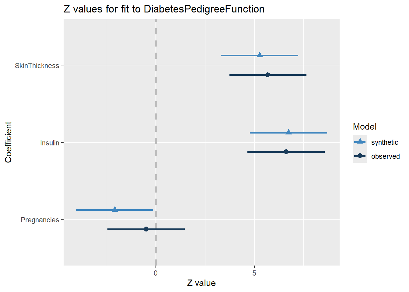
Fairly similar results, but there appears to be more variation than the previous comparison
Next, we can assess correlation as a whole.
rawdatacor = cor(rawdata[1:9]) # Original dataset correlation between variables
synthdatacor = cor(synthetic_data$syn[1:9]) # Synthetic dataset correlation
corrplot(rawdatacor)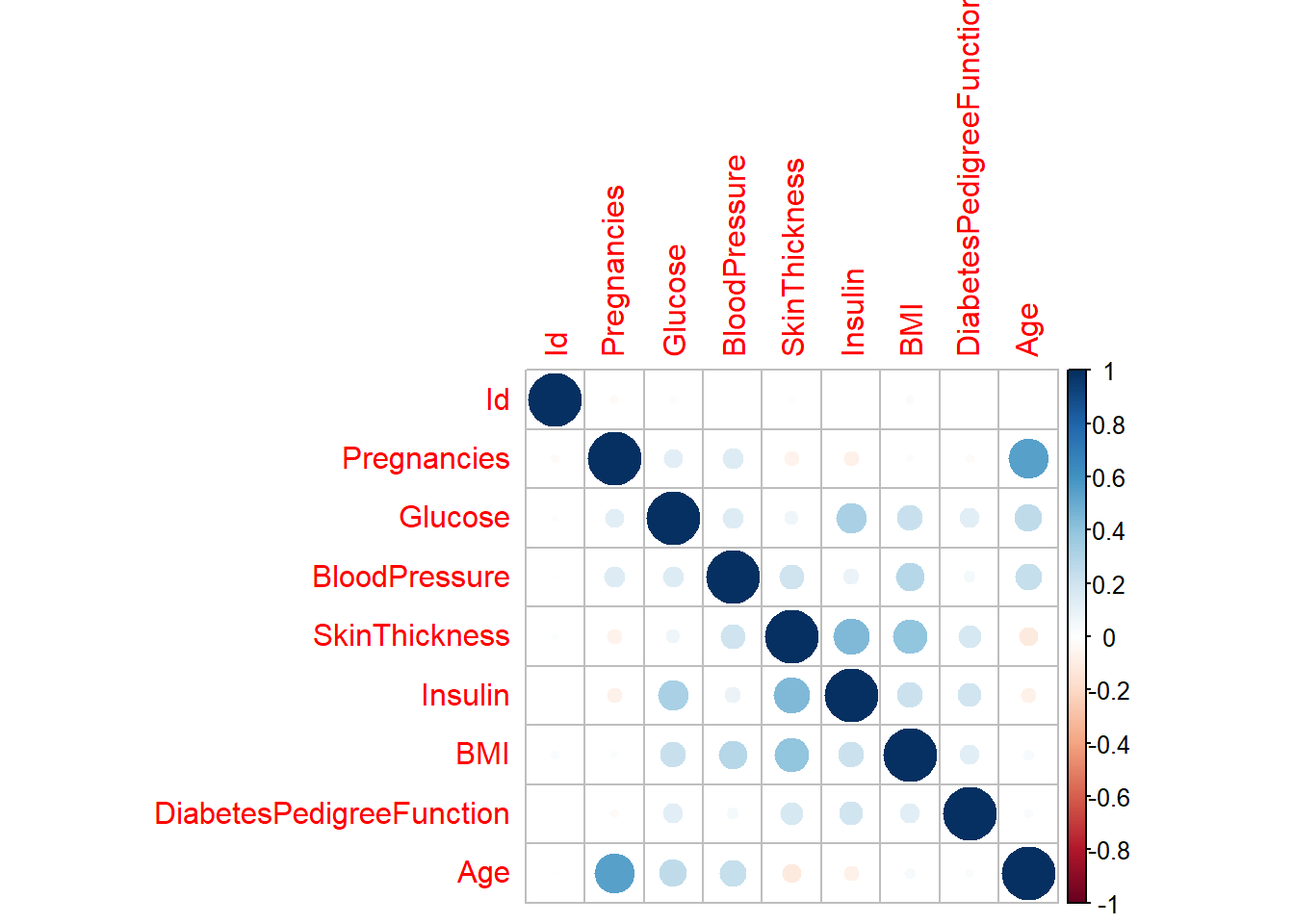
corrplot(synthdatacor)
We can see that these two correlation plots are virtual identical, indicating that the associations between variables stayed the same across the new data set.
Conclusions
Overall, we can conclude that our new synthetic data set maintains the same shape and spread as our original data set while maintaining key associations between variables. If the original data set were a true data from real patients, we have now created an anonymized dataset that can now be used for further analysis.